Color – Part Two – The Hanna Formation

So, now that I’ve explained color in yesterday’s post, let’s see what some geological data look like.

These are ugly graphs of raw data constructed in Excel. I wouldn’t publish these, but we can use them to visualize the data at a first pass.

Let’s start in the Hanna Basin. This summer, my field assistant and I measured the rock thickness and took color measurements with the RM200QC in a critical part of the Hanna Formation that most likely includes the Paleocene-Eocene boundary (55 million years ago). You can see the travelogues for those days in the field here and here.

It was a little over 150m of rock thickness that we measured in two parts. We began the measurement at the top of a series of lake beds we call the lower lacustrine unit (LLU), went through a river-deposited section, the fluvial unit (FLU), and into another series of lake beds called the upper lacustrine unit (ULU).

Here’s the results from the first part. This goes all the way from the LLU into the ULU.

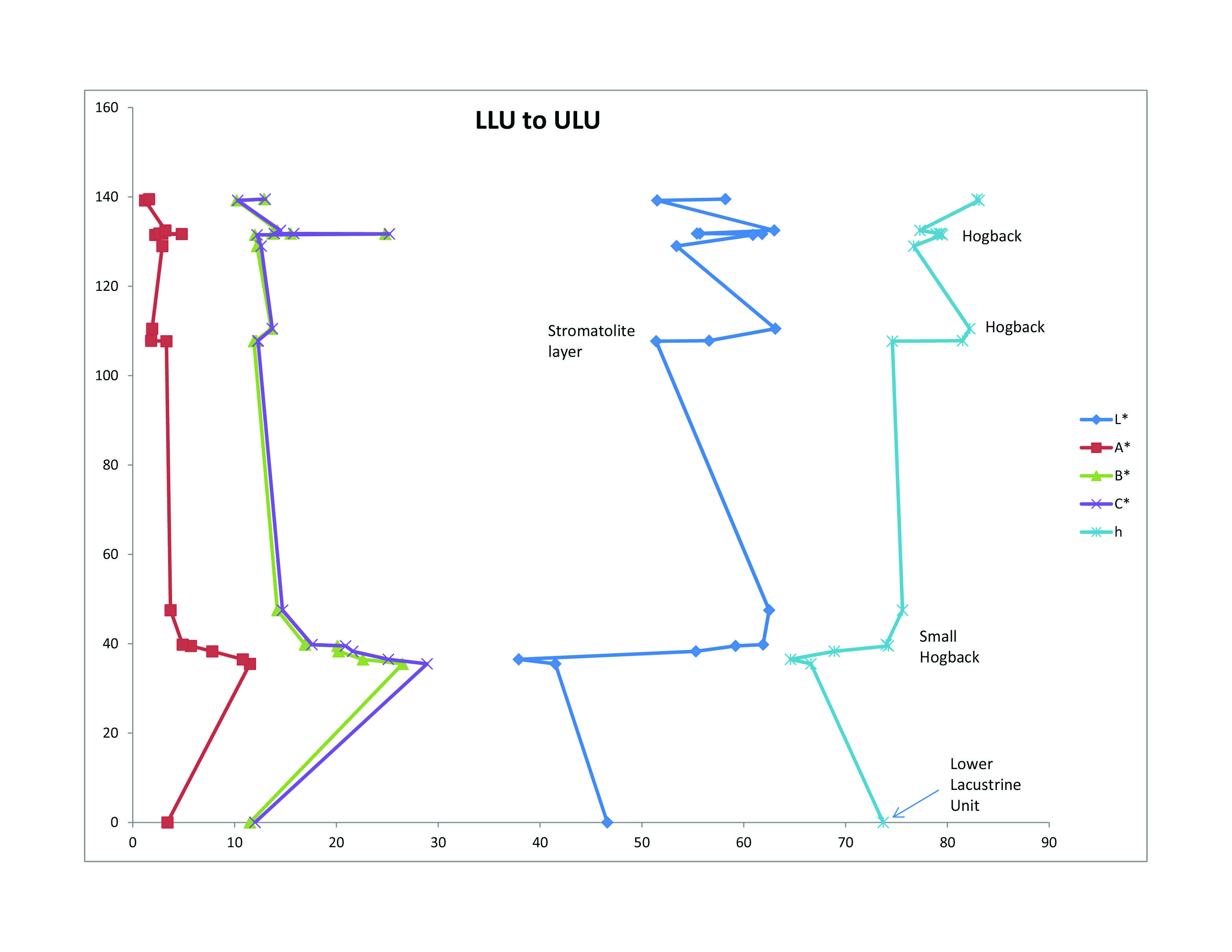
A lot of the section was covered. That is to say, the rocks weren’t exposed. Rather they were hidden by soils and foliage. Thus, we don’t have continuous data. We have big gaps between ~50 and ~100 meters (the vertical scale) and also between the LLU and 30 meters.

But there are some patterns. Rocks are often exposed in little hogback ridges. At each hogback, there is a positive trend in L* and a negative trend in a*, L* and a* being the two most commonly used color parameters in professional papers.

We moved over a bit and re-measured the section starting at about ~130 meters, where there is an easily traceable layer of stromatolites.

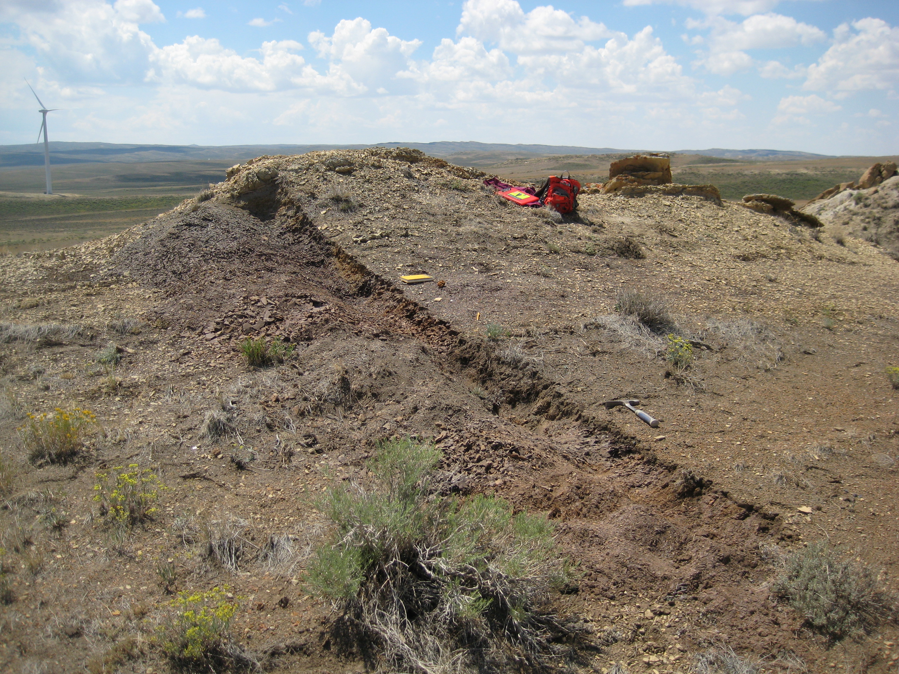
Stromatolites are the fossil remains of algal mats or domes. The presence of stromatolites tells us we are in a lake environment. We moved over to re-measure because the exposures were better, there were some more stromatolites, and we could tie in an important fossil-bearing layer (the ‘flower bed’) from which I collected a fossil flower many years ago. We thought we could get a more complete record this way.

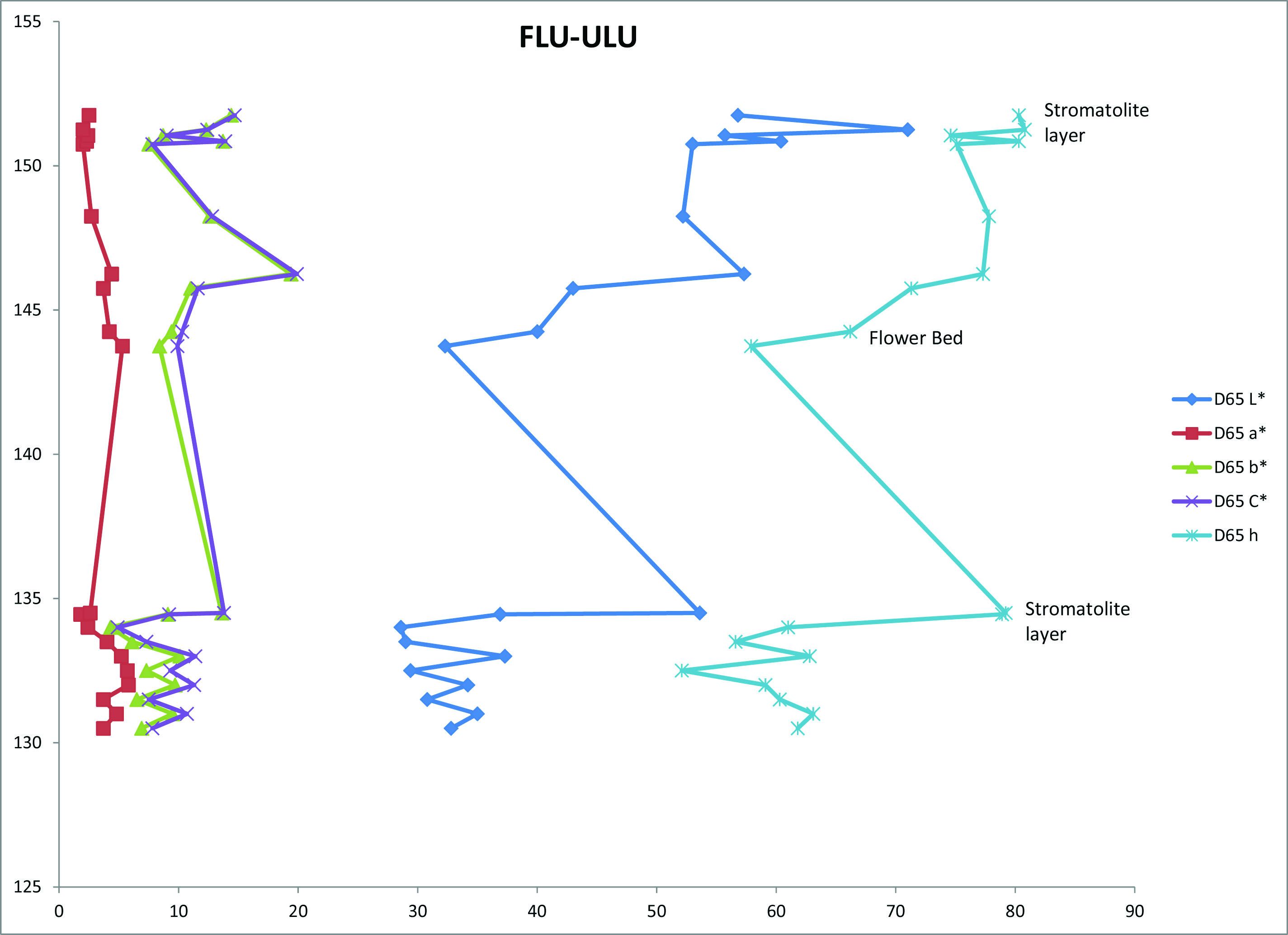
The same pattern holds true here, with a positive shift in L* at hogbacks (where there are also stromatolite layers), and a negative shift in a*.

Below, I’ve stacked the two plots together, so you can see how they relate.

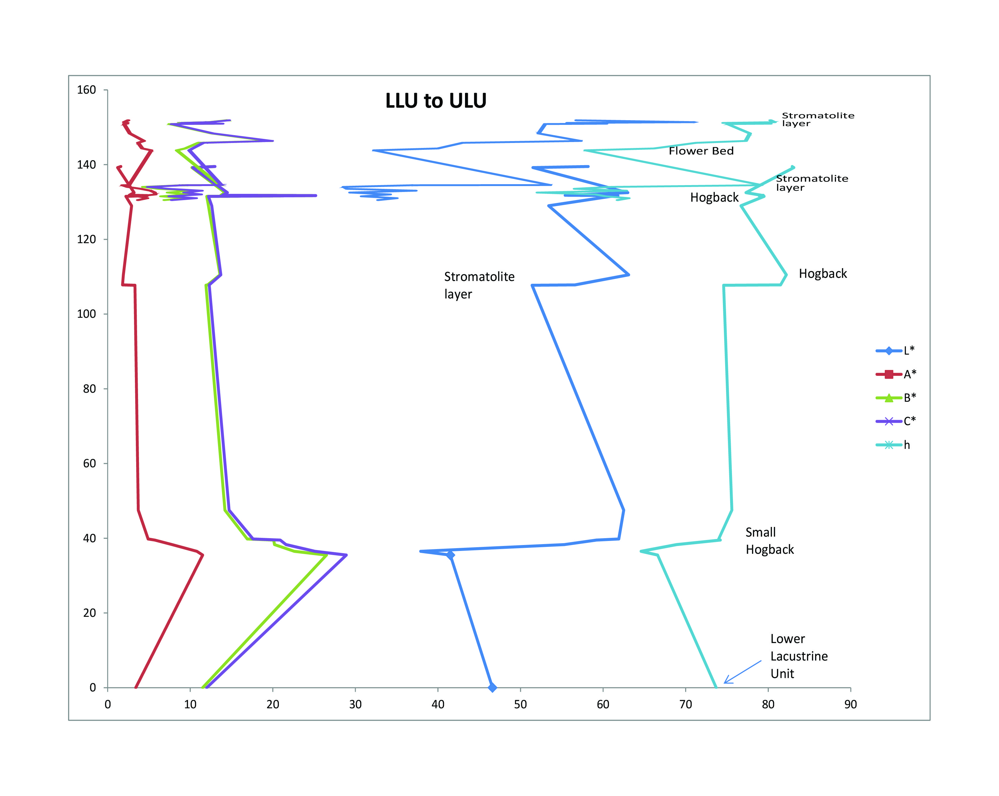
Now what? We see this pattern. What does it mean? I suspect that this may be due to orbital patterns like I describe here in relation to modern global warming. I think the repeating pattern of hogbacks with stromatolites might represent a 20,000 year cycle.

Do you have any thoughts?

A few things have come out of this. Most importantly: color analysis works.

We’ll most likely be coming back with a color analyzer next summer, but with a focus more on lower parts of the Hanna Formation, below the LLU. The rocks there also have a repeating pattern of sandstone hogbacks with finer-grained mudstones in between, all of which were deposited in a river environment. I want to see if there is any cyclicity to that, among other things.

So, here’s the data. We have to make sense of it now, or decide what further steps need to be taken to make sense of it. This is a preliminary dataset, so I don’t expect grand conclusions at this point.

But maybe there is some grand conclusion to be made from this. Does anything jump out at you? Do you see something that I’ve overlooked?

This is the process of science. Please, feel free to participate.